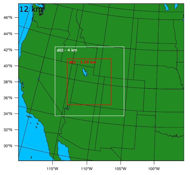
The goal of this research project is to move toward the improved modeling of wintertime persistent cold air pools in Utah.
The study currently focuses on three basins within Utah: the Salt Lake Valley, the Uintah Basin, and the Cache Valley.
In order to reach these goals, a number of WRF model runs were carried out and various 'sensitivity tests' were performed in
order to determine which changes we made to the WRF model improved its overall performance.
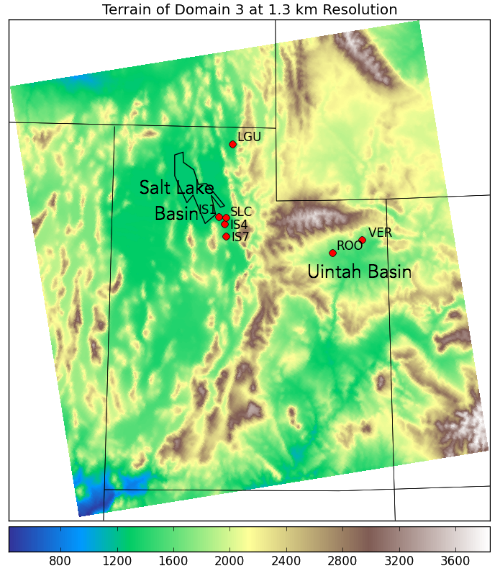 Figure 1.
 Terrain of innermost domain 3, overlayed with station locations used for
validation in this modeling study.
Various land use classification schemes were tested because of the known link between land use category and albedo, which plays
a major role in the life cycle of persistent cold-air pools through its interaction with model snow cover. Three land use data
sets were compared in relation to their influence on the modeling of PCAPs IOP5, 1-9 January, 2011. Some results of this
sensitivity study follow.
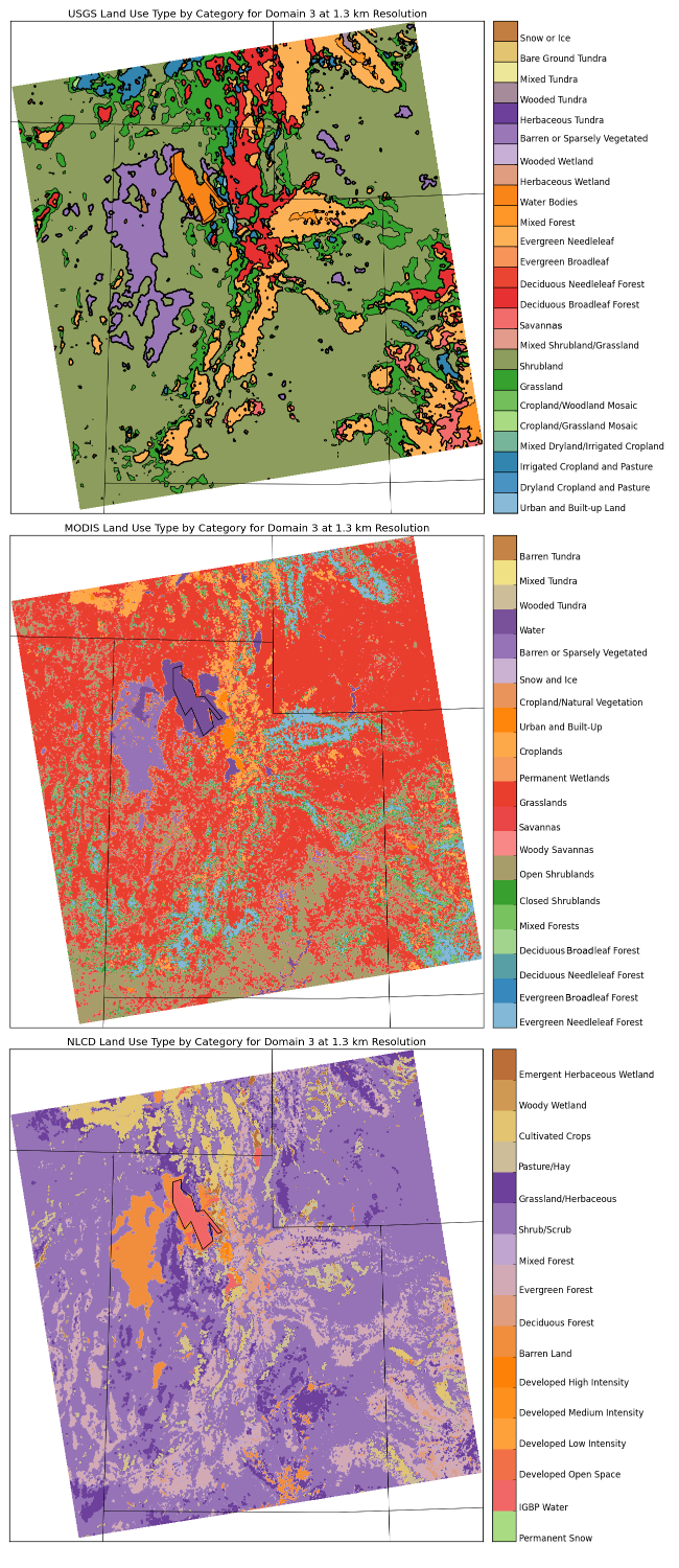 Figure 3.
 Maps of land use type by category for WRF model domain 3.
Pictured are those of USGS, MODIS, and NLCD land use respectively.
Figure 3 emphasizes the striking disparities between model land use categorization schemes and thus the need to fully understand how these
differences interact with the modeling of cold air pools in Utah's basins. Considering the geographical differences between the three basins of
interest to this study, it seems beneficial to examine (qualitatively) the differences in land use for each.
Salt Lake Basin:
 Figure 4.
 Summary of Great Salt Lake elevation
(source).
The elevation of the Great Salt Lake varies from year to year depending on the precipitation its watershed receives. In 2011, the lake's elevation was
4196.1 feet above sea level, nearly 6 feet below the average level shown in Figure 4. This would mean the lake's shoreline exists somewhere between that
of the average and historic low. While USGS and NLCD land use schemes capture this feature relatively well, the MODIS classification currently used by WRF
does not. It's lake level more closely resembles that of the historic high period, which is because the MODIS data used in this classification scheme
is from a time when the Great Salt Lake level was above average.
Since the Salt Lake Basin consists of the Salt Lake Valley (to the southeast), as well as the area encompassing the lake itself, the resulting implications
of incorrect lake size on the modeling of cold air pools are numerous. Some of these include:
- Inaccurate land-atmosphere interactions, since 'lake' exists in the model where it shouldn't (when usings MODIS).
- Inaccurate albedo (which plays a significant role in cold air pool strength), since snow cannot exist on lake surface.
Uintah Basin:
All three land use categorization schemes classify the majority of the Uinta Basin as shrubland or grassland, which in itself isn't a large disparity. The issue
arises from how these classifications interact with the snow cover produced by the model, which in turn presents a number of issues that need addressing. Depending on
whether or not the model treats a certain snow depth (or SWE) as either fully covering the vegetation or not, the resulting albedo is influenced significantly. In WRF,
this is represented by the variable, SNUP, which is defined as the threshold depth or equivalent SWE for 100% snow cover. Even if the model produces accurate snow depth,
if it's not then converting this into an albedo representative of truth, the cold air pool will respond accordingly. (Higher albedo results in less short wave absorption,
thus less long wave emission and warming of the atmosphere, ultimately allwoing the inversion imposed by the cold air pool to sharpen.)
Another issue simply stems from how effectively the snow covers the vegetation in the model as compared to known conditions within the basin. If the land use scheme
equates snow covered grass or shrubery to a lower albedo (think dispersive bunches of grass that spread out above the snow), when in reality the vegetation might not even
reach too far above it. Figure 5 illustrates an example disparity, which was found to be true of WRF model runs done by Erik Neemann of a cold air pool that occured
in the Uintah Basin during
February of 2013.
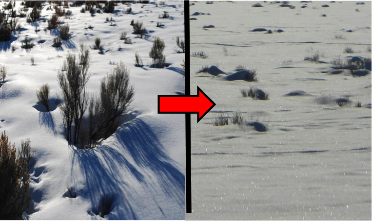 Figure 5.
 Left: possible WRF treatment of vegetation before modification.
Right: observed vegetation and its true impact on albedo.
Initial Findings of Land Use Sensitivity WRF Model Runs:
Figure 6 shows how changing only the land use scheme (from USGS to MODIS) can impact the albedo of more sensitive areas (i.e. water bodies and valleys prone to snow cover).
The largest differences are located around several Utah lakes, most notably the Great Salt Lake, Utah Lake, and Bear Lake, and at higher elevations along the Wasatch Front.
Albedo differences of +0.5 (and greater) saturate the area surrounding the Great Salt Lake where in the MODIS land use scheme there exists lake, but in the USGS scheme there
does not. The sign of this value is significant because a positive (negative) value refers to the USGS (MODIS) run having a higher average albedo over the nine day model run.
This makes sense, considering water has a lower albedo than barren/sparesly vegated land and cannot exist with snow cover, unlike the latter.
Less pronouced (due to the extreme values imposed by the differences in lake perimeter between schemes) is the albedo differences present in the Uintah Basin. Overall the
basin seems to have higher albedos in the USGS run than the MODIS run. This difference is further highlighted in Figure 7, which is the same plot as Figure 6, only average
two meter temperature is being differenced, not albedo. Therefore, positive (negative) values mean the USGS (MODIS) run is on average warmer than the other. At lower elevations
within the Uintah Basin the temperature difference is predominantly negative, meaning the USGS run (which had higher albedos) is on average cooler than the MODIS run. This
relationship between albedo and temperature is better observed in the areas surrounding the Great Salt Lake, Utah Lake, and Bear Lake.
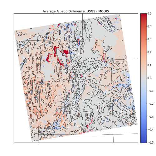 Figure 6.
 Average albedo of domain 3 from 1-9 Jan 2011, USGS run minus MODIS run.
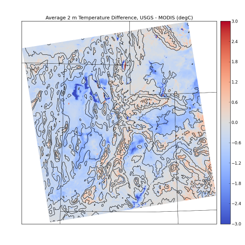 Figure 7.
 Average 2 m temperature of domain 3 from 1-9 Jan 2011, USGS run minus MODIS run.
Figures 8 and 9, while initially meant to compare the three land use runs to observations, as well as each other, also shed light on WRF's ability to model cold air pools in
Utah's varying basins. Figure 8 shows decent agreement between each model run and observations at the SLC surface station (located at the SLC Airport). Simply in reference to
this, there's no clear advantage to each of the three land use schemes. They all capture the dirunal pattern relatively well and although they tended to amiplify the temperature
range experienced on certain days, which suggests the model didn't fully produce a cold air pool as strong as the one observed, Figure 10 shows that it at least did form a cold
air pool within the Salt Lake Valley during this time period (IOP5).
Figure 9, on the other hand, shows an obvious disagreement between modeled and observed temperature for a surface site in the Uintah Basin. The temperature of each run at model
hour 0 was roughly 5 degrees warmer than observation, a difference that only increased over time. The models appear to capture a week dirunal cycle over the first three days,
but this is even lost past hour 72, when the temperature disparity between model and observation begins to exceed 10 degrees. It is thought that this transition into an extended
period of weak diurnal variation is the result of the model producing cloud cover within the Uintah Basin, when in reality this was a cloud free case. In terms of land use
sensitivity, there does appear to be consistent differences between the three runs. The USGS run produced the coldest temperatures at VER throughout the entirety of the run and
while this difference never exceeded a degree or two when compared to the warmer NLCD run, it was one of the factors taken into account when choosing the USGS land use scheme
for future sensitivity studies.
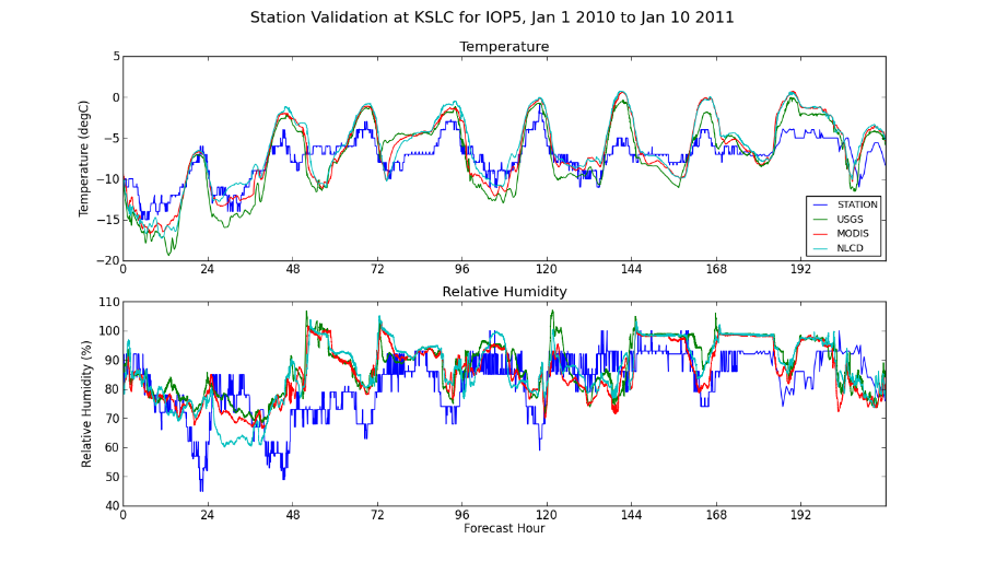 Figure 8.
 Time series of temperature and relative humidity at Salt Lake City (SLC)
from observations and USGS, MODIS, and NLCD WRF model runs.
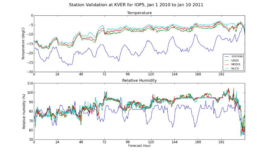 Figure 9.
 Time series of temperature and relative humidity at Vernal (VER)
from observations and USGS, MODIS, and NLCD WRF model runs.
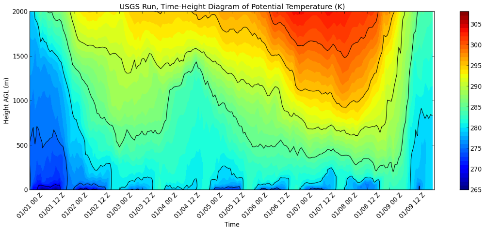 Figure 10.
 Time-height diagram of potential temperature in the Salt Lake basin for the USGS run from 1-9 Jan 2011.
Pictured are the first 20 vertical levels from the WRF model run. Black contours are plotted every 5 K.
Considering the disparity between the models' initial
Figure 3. Maps of land use type by category for WRF model domain 3.
Pictured are those of USGS, MODIS, and NLCD land use respectively.